7 Steps to Create the Perfect Formula, Every Time!

In the previous edition of The Dossier, we debunked the Excel Myth: “… to be skilled at using Excel, you must be a math head”.

Now I will share with you, my proven recipe for creating the perfect formula – every time. The recipe works no matter whether the formula is simple or complex.

Secret recipe, DEFCORE:

Destination Cell
Equals Sign “=”
First Cell
Calculation Sign (, *, /, +, -, ^, )
Other cell
Repeat Steps 4-5 until complete
Enter or Tick

1) Destination Cell

Move the cursor to the destination cell.

I know – this sounds obvious – but I have seen many times where students of Excel (and Pro users too) become so fixated with the formula they are about to create that they don’t even notice where the cursor is when they start typing.

That’s a sure-fire way to over-type something important – if you don’t think about it first.

That’s why I added this step!

2) Equals “=”

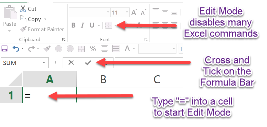
Every formula in Excel starts with an “=” sign – no exception! As soon as you type this symbol, Excel immediately knows that what follows is to be calculated.

By typing the “=” symbol, Excel changes from Cell Mode to Edit Mode. This can be identified by the Cross and the Tick symbols which appear on the Formula Bar.

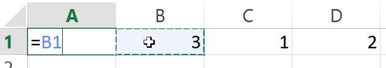
equals, excel, edit mode, cell mode — *Figure 1: Type the “=” sign to start the formula*

3) First Cell

When creating a formula in Excel, you can either type the cell reference (e.g. “B5”) or you can use the mouse and click on the cell. Using the mouse is called the “Point and Shoot” method – because by clicking on the cell, the cell reference appears in the formula.

The Point and Shoot method is my preference because it removes the line of sight errors when you are working out the cell reference coordinates. It is much safer to click on the cell you want and Excel will insert the reference for you.

excel, point and shoot, formula — *Figure 2: Use the Point and Shoot method to select cell B1*

4) Calculation Sign

Step 4 is where we tell Excel what type of calculation to perform. The options are:

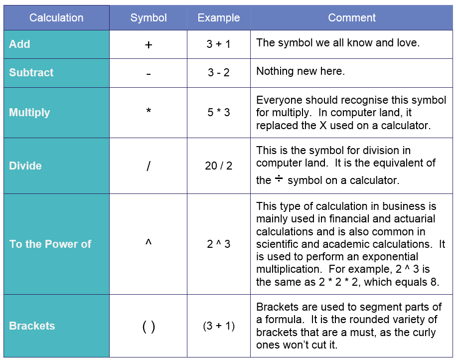
You can use these calculation symbols as many times as you like in a formula.

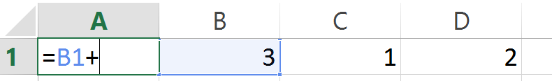
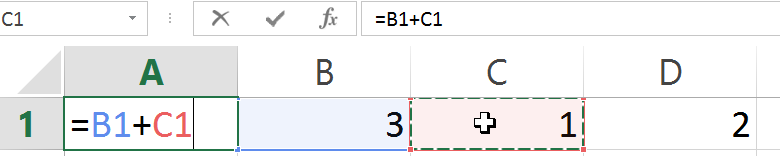
In this case, we want to use the “+” calculation. So type the “+” as shown below:

Excel Perfect Formula Figure 3 — *Figure 3: Type the “+” symbol to tell Excel we want to add values*

5) Other Cell

In this step, you use the Point and Shoot method to select the next cell in the formula.

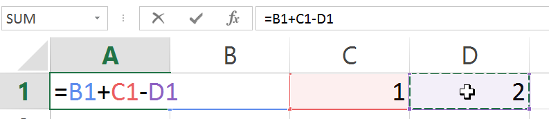
excel, formulas, point and shoot, DEFCORE — *Figure 4: Click on the next cell to add to the formula*

6) Repeat Steps 4-5

Depending on the complexity and the length of the formula you may not need this step, and you can proceed straight to Step 7.0. If, however, the formula is longer and involves more calculations or cells, it is simply a matter of repeating Steps 4 and 5 until you have included all calculations and cell references.

Something to note – your formula should always end with a cell reference or a Bracket. Never finish with a Calculation Symbol [+, -, *, /, ^]. Otherwise, Excel will complain about it loudly.

excel, formulas, DEFCORE, calculation, calculation signs — *Figure 5: Type the “-” and click on cell D1 to complete the calculation*

7) Enter or Tick

The final step in creating the formula is to “lock it in” and return to Cell Mode.

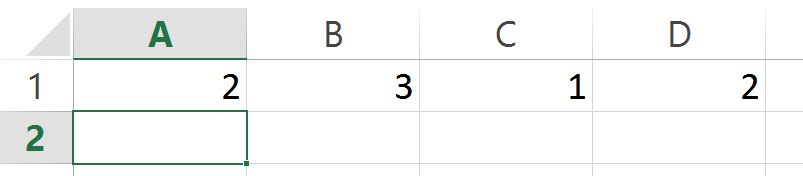
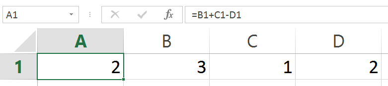
excel, DEFCORE, calculations, formula — *Figure 6: Press the Enter key to “lock in” the formula and return to Cell Mode*

excel, calculations, formula, DEFCORE — *Figure 7: Click back onto the Destination Cell to see the formula displayed in the Formula Bar*

Voilà – all done!

That is the DEFCORE secret recipe for creating the perfect formula – every time!

Watch out for our next article as we examine the internal rules that Excel uses to calculate the result of your formula – this may surprise you!