
Using Microsoft Excel is something that people either LOVE or HATE. And the only difference between those two kinds of people is whether you understand it or not.
Let’s pretend you’re the owner of SellingCoolStuff Pty Ltd and you have four salespeople who work for you: Bob, Jane, Mary and Fred, and you want to use Excel to track the total sales that each of them has made in the previous week.
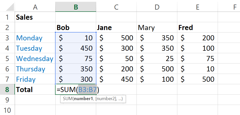
In the above image, I simply clicked the AutoSum function to total the figures in Column A. To get the totals for Jane, Mary and Fred, you can then copy this formula to Column B and C.
This is called Relative Cell Referencing (ooooooohhh, fancy!). It’s Excel’s default cell referencing, which it does without you having to modify the formula.
Let’s see what happens when you click and drag the sum from Column A over to Column E.

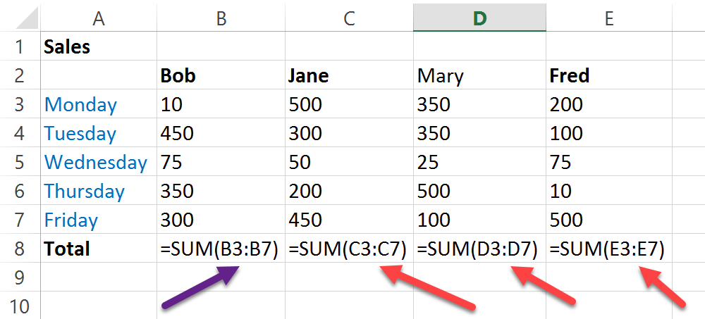
Sweet! See how when the formula was copied from Column A to Column B, the formula now shows the total for Jane’s week, instead of Bob’s? It also shows the correct cell references for the position of the formula. i.e. “B” changes to “C”, then “D” and finally “E”.
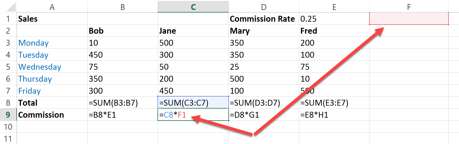
Now let’s consider another scenario. Let’s assume that we want to calculate the commission for each sales rep in the example below.
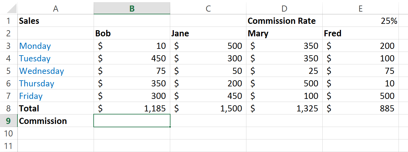
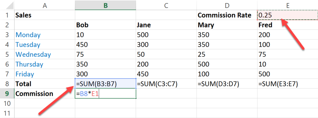
Each sales rep will receive 25% of their sales figure for the week as a commission (let’s keep it simple). So, the formula for calculating Bob’s commission will be B8*E1:
Straight forward so far. But is it?
Do the same thing as with the sums and copy the formula across to Fred’s column. Notice what happens:

Huh? What happen there? Excel has applied Relative Cell Referencing to the formula as it has been copied. Such that Jane’s sales figure is being multiplied by an empty cell (F1) which is the same outcome for Mary (G1) and Fred (H1). No wonder, their commission was zero. So how do we fix that WITHOUT typing the 25% figure into the formula? Easy!
The Fix?
- To fix this we need apply Absolute Cell Referencing:
- Return to the original formula and examine the cells referenced in the formula.
- In Bob’s example, we have B8 and E1.
- Ask yourself – which cell or cells needs to remain the same after the formula has been copied?
- Your answer should be E1.
- Click on the formula bar and place your cursor between the E and the 1.
- Press the F4 key on the keyboard and $ signs will appear in front of the E and 1, as shown:
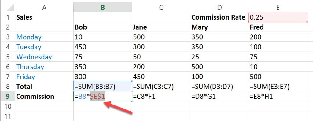
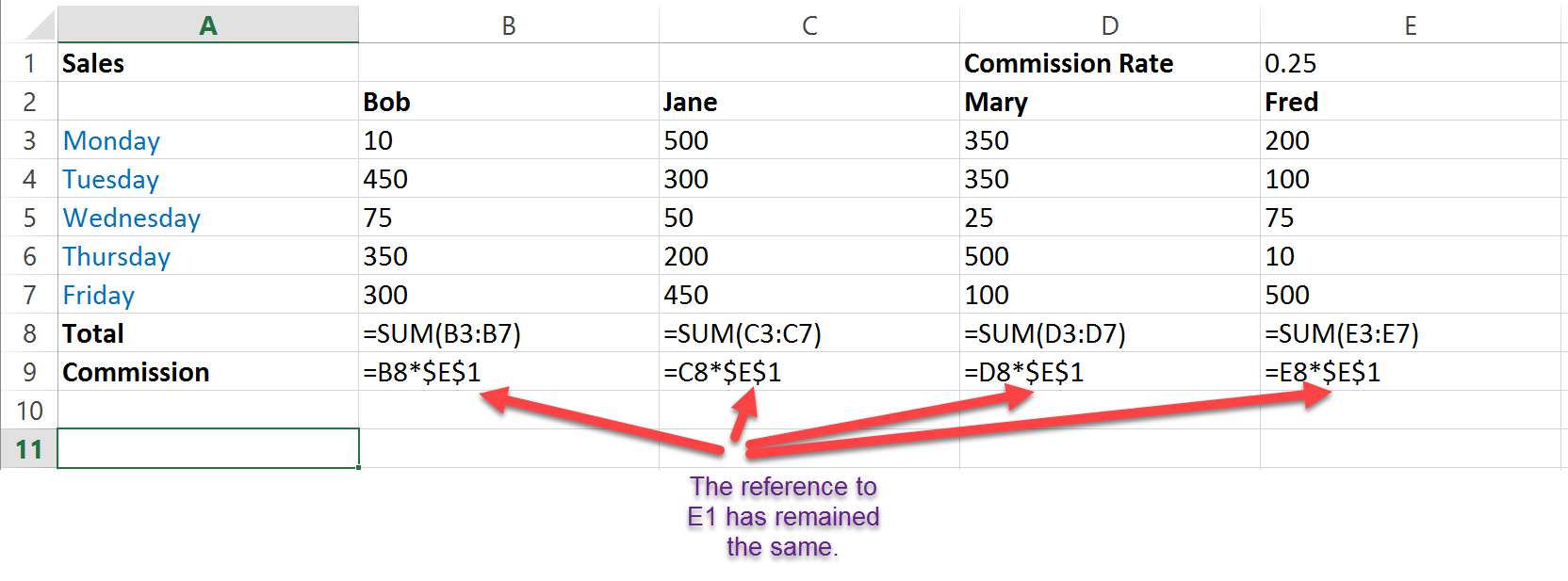
Apply Absolute Cell Referencing to stop the commission rate changing as the formula is copied. In this case, the $ signs do not mean currency. Instead, they mean, keep this cell reference no matter what.
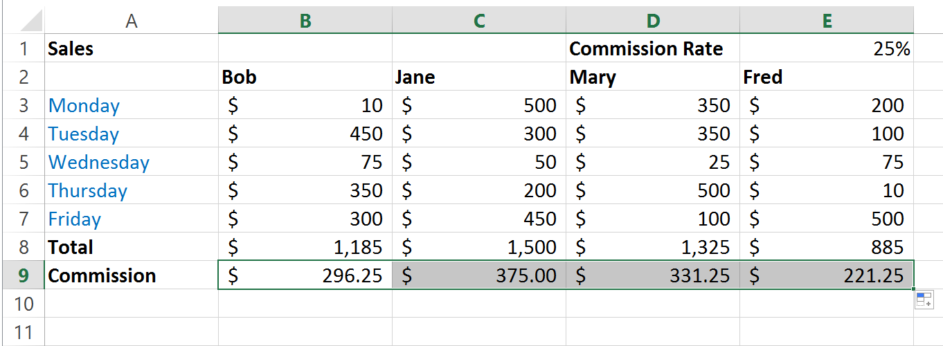
- Lock in the formula by pressing the Enter key.
- Then copy the formula again and notice the difference!
Other fun facts
There are other variations of Absolute Cell Referencing, which can be found by continuing to press the F4 key.
Relative Column / Absolute Row – ![]()
Absolute Column / Relative Row – ![]()
Relative Column / Relative Row – ![]()
Which can all be used for various purposes that we can cover another time. Great job for today!!
Quiz
Before I go, I will leave you with a brain teaser! See if you can work out how to complete this puzzle:
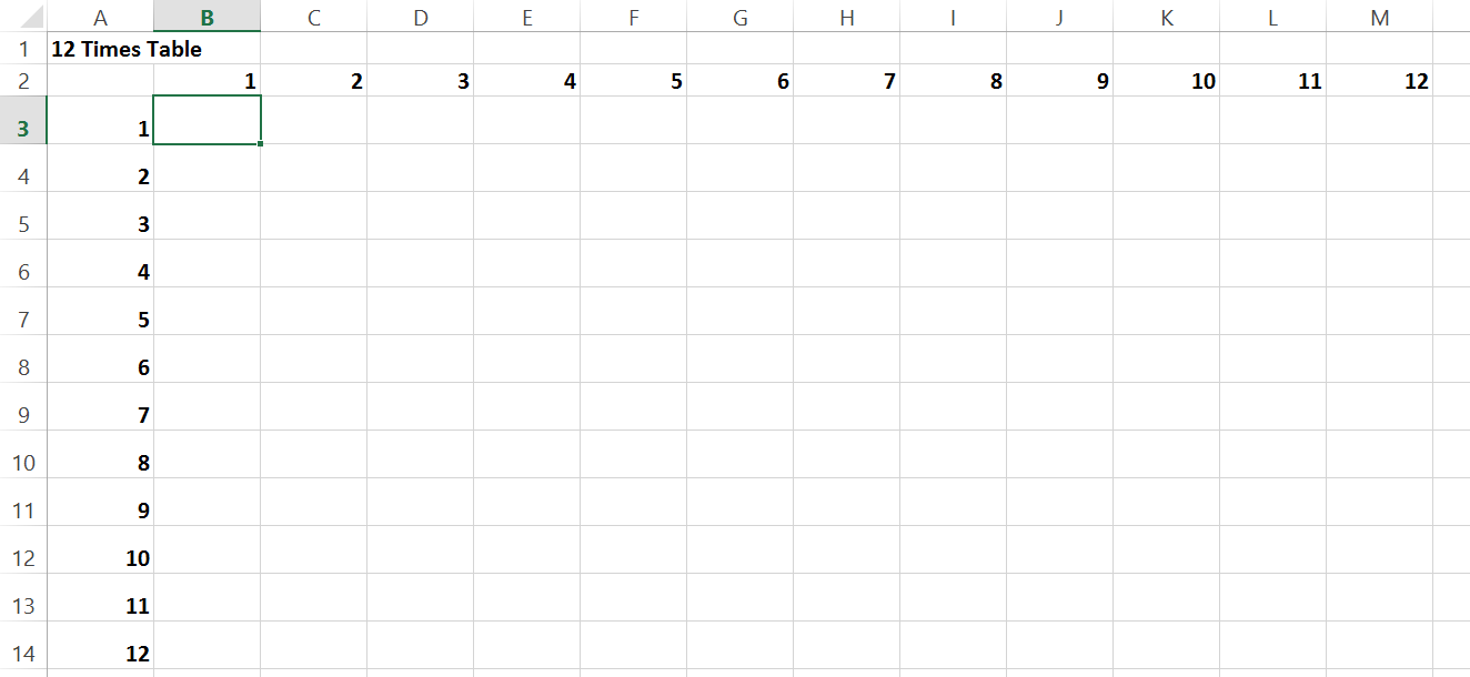
See if you can use your new Cell Referencing knowledge to work out the required formula.
Rules:
- Finish the 12-Times Table.
- Using only one formula placed into cell B3.
- Copy that formula down and then across or across and then down to complete the table.
- Remember – ONE FORMULA ONLY!
I will share the answer in the next Excel article.
Leave a Reply
You must be logged in to post a comment.