Excel Magic – the Payment Function (PMT)

I will assume most of us have had a loan or mortgage or, if not, you’ve probably at least contemplated one. You know the drill. You see something you like on realestate.com, head to the slick calculators on the website of your chosen financial institution and either give yourself a fright or leave wondering about the transparency of the calculator.

To teach you a bit more about the magic of Excel, I’m going to use the idea of this calculator to learn about a really cool function within spreadsheets… It will probably even impress people who use Excel all the time!

The Payment (PMT) Function

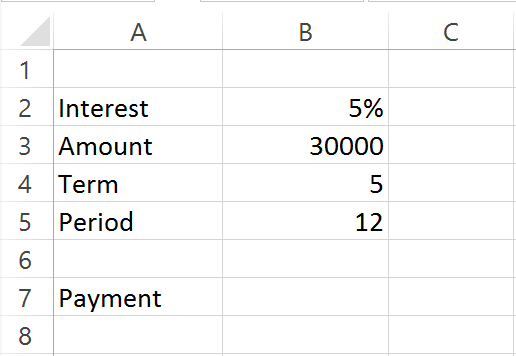
Let’s start with some figures in an Excel spreadsheet. Let’s imagine you want to take out a loan to buy yourself a new car.

In this case, we want to calculate the monthly repayment on a $30,000 principle.

Step 1: Creating the Formula

• Select the Formulas Tab on the Ribbon.
• Click on the Financial Functions drop-down
• Select PMT.

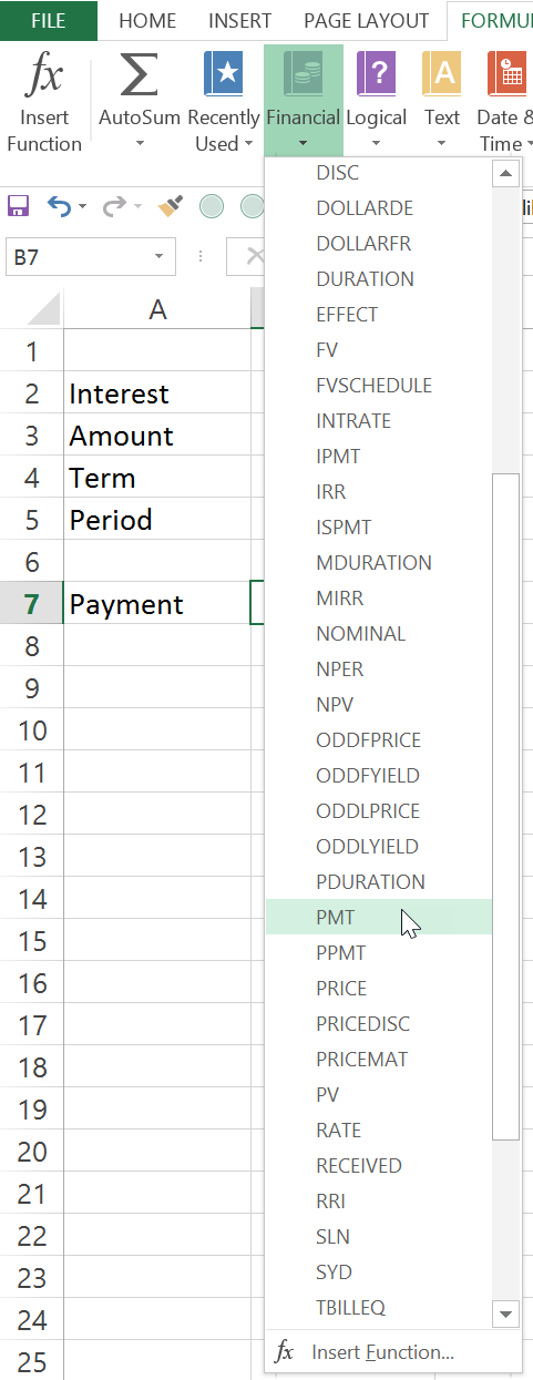
• The Function dialog box will open, displaying the arguments of the PMT formula:

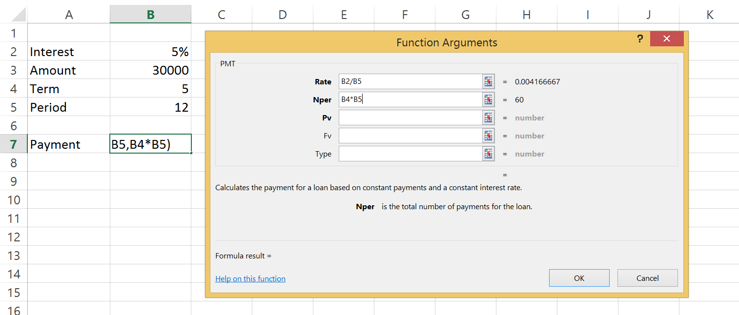
Step 2: Enter the Rate

The first Argument to enter is the Rate. Ensure that the cursor is in the Rate text box and then

• Click in cell B2. The interest rate is a per annum rate so we need to convert this to a percentage that will match the Period value.
• Type a “/” for divide.
• Click in the cell B5 and the Rate Argument will look like this:

Step 3: Enter the number of periods

The next argument is Nper – which means the total number of periods.  Given the term is 5 years and there are 12 payments in a year we need to multiply the Term value by the Period value to give us the Nper. (It’s okay, don’t go cross-eyed on us just yet, you’re doing great!)

• Click in the Nper text box.
• Now click in the cell B5.
• Type a “*” for multiply
• Click in cell B5 and the Nper text box should look like this:

Step 4: Enter the Present Value

The next argument to be completed is Pv – which stands for Present Value.  It is the amount that will be borrowed… in this case $30,000

• Click into the PV text box.
• Then click into cell B3.
• In this example, we will leave the last two arguments blank:

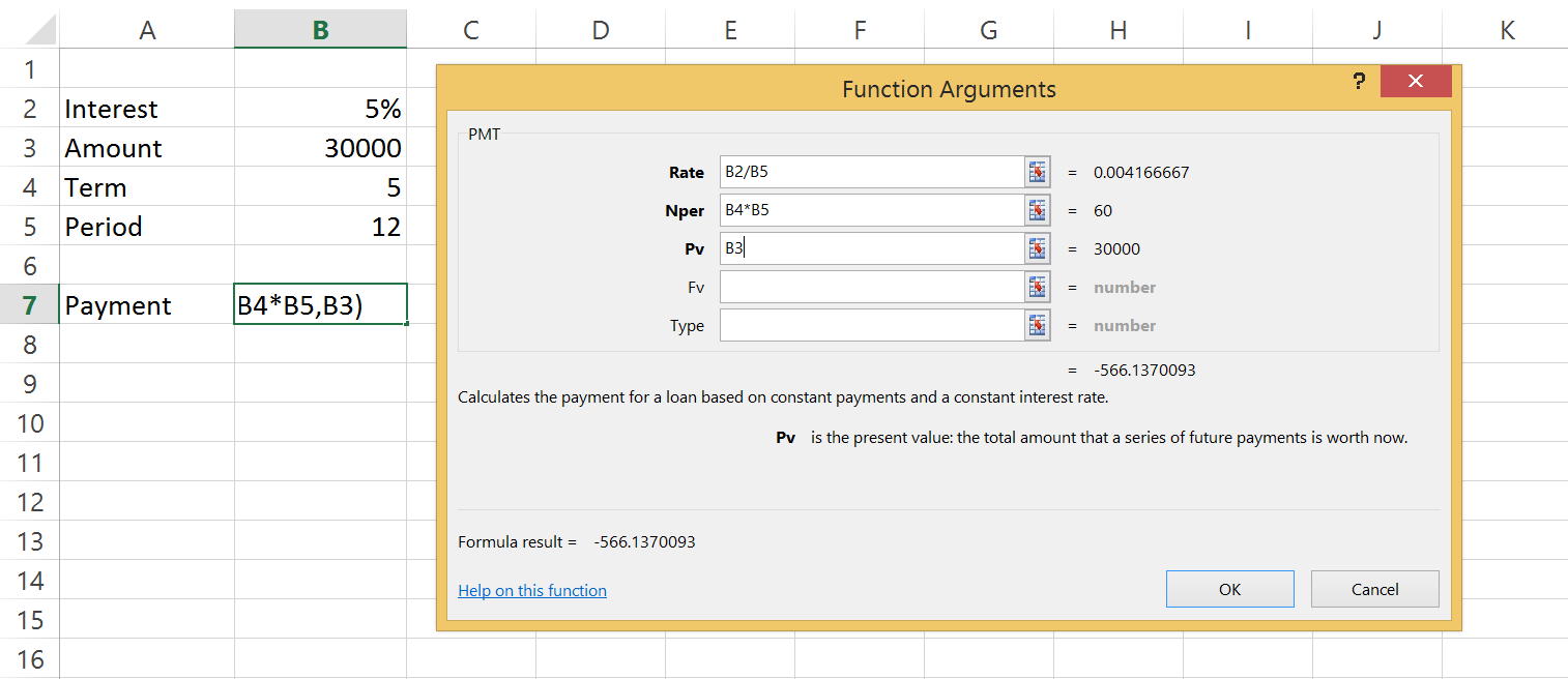
Fv – Future value, we will assume that we will pay the loan out completely, therefore leaving the text box blank equates to zero.  If the loan has a balloon figure at the end of the loan you would enter the balloon value in this text box.

Type – This text box determines whether the interest is calculated at the end of the period or at the beginning.  Entering a zero, or leaving the field blank indicates the interest is calculated at the end of the period.  While entering a 1 will ensure the interest is calculated at the beginning of the period.

Step 5: Calculate

• Click OK to complete the function and display the answer.

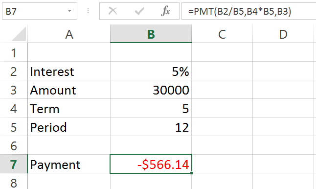
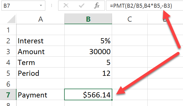
• Notice, the result is a negative value.  This is because Excel treats this as an outgoing payment.  If you want to change this to a positive figure modify the function to put a minus sign in front of the Pv argument, like this:

Too easy!  Now you can play with values in the cells. To see what the repayments would be if you changed the:

• Period to fortnightly (26).
• Increased or decreased the Amount borrowed.
• Increased or decreased the Term.

Want to really scare yourself?

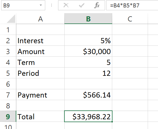
If you want to see something really scary – calculate the total amount repaid over the term:

Put this formula in cell B9, = B4*B5*B7

That’s if for the PMT function.  Join me in the next article when we look at another handy tip about Excel!